Plotting with TikZ, Part III: Plotting a function defined by a formula, and plotting functions that go through certain points

2019-05-13T15:41-05:00

TikZ ist kein Zeichenprogramm, indeed, LaTeX, math

In the last post, I described how I use TikZ to create a graph that might otherwise be created freehand:

In this post, I will describe one method for using TikZ to to plot a function defined by a formula, such as $$y = \left(2x^2 - x - 1\right)e^{-x}.$$ Then I will show two ways to make a function go through a certain point.

Plotting from a formula

Simple example

There are a number of ways to achieve this, and PGF actually includes the functionality to perform calculations in TeX. (For example, I have used the PGF pseudorandom number generator in graphics. Someone even made TikZ code to generate a random city skyline.) However, for efficiency sake, I prefer to have the calculations done outside TeX, in a more efficient computer language.

The trick is to use the gnuplot table import format. You simply have to generate a text file with a list of coordinates in the following form:

-1.250000 11.779907
-1.240000 11.456050
-1.230000 11.138839

This file contains the coordinates $(-1.25, 11.779907)$, $(-1.24, 11.456050)$, $(-1.23, 11.138839)$.

There are a number of ways to generate such a file. Since I like Python, I used the following (simple) Python script:

 1
 2
 3
 4
 5
 6
 7
 8
 9
10
11
#! /usr/bin/env python3

import numpy as np

f = lambda x: (2*x**2 - x - 1)*np.exp(-x)

xvals = np.arange(-1.25, 10.25, 0.01)

with open("plot1.table", "wt") as outfile:
    for x in xvals:
        outfile.write("{:f} {:f}\n".format(x, f(x)))

Now, this curve can be imported into your TikZ illustration using \draw […] plot; in this case:

\draw[thick, blue, <->] plot[smooth] file {plot1.table};

Here is a complete example (with coordinate axes and everything):

 1
 2
 3
 4
 5
 6
 7
 8
 9
10
11
12
13
14
15
16
17
18
19
20
21
22
23
24
25
26
27
28
29
30
31
32
33
34
\documentclass[border=0.25cm]{standalone}

\usepackage{tikz}
\usepackage{fouriernc}

\begin{document}

  \begin{tikzpicture}[yscale=0.5]

    \draw[gray] (-1.25, -1.25) grid (10.25, 12.25);

    % x-axis
    \draw[thick, black, ->] (-1.25, 0) -- (10.25, 0)
      node[anchor=south west] {$x$};

    % x-axis tick marks
    \foreach \x in {-1, 10}
      \draw[thick] (\x, 0.2) -- (\x, -0.2)
        node[anchor=north] {\(\x\)};

    % y-axis
    \draw[thick, black, ->] (0, -1.25) -- (0, 12.25)
      node[anchor=south west] {$y$};

    % y-axis tick marks
    \foreach \y in {-1, 12}
      \draw[thick] (-0.1, \y) -- (0.1, \y)
        node[anchor=west] {\(\y\)};

    % graph of function
    \draw[thick, blue, <->] plot[smooth] file {plot1.table};

  \end{tikzpicture}
\end{document}

And here is the output:

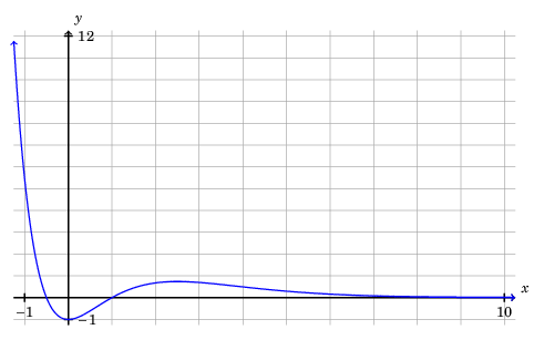
In my Python script above, I carefully chose the set of inputs $x$ (np.arange(-1.25, 10.25, 0.01), i.e., every real number of the form $-1.25 + 0.01k, \; k \in \mathbb{Z}$ in the interval $[-1.25, 10.25)$) to keep $f(x) < 12$. This can also be handled computationally.

Example involving asymptotes

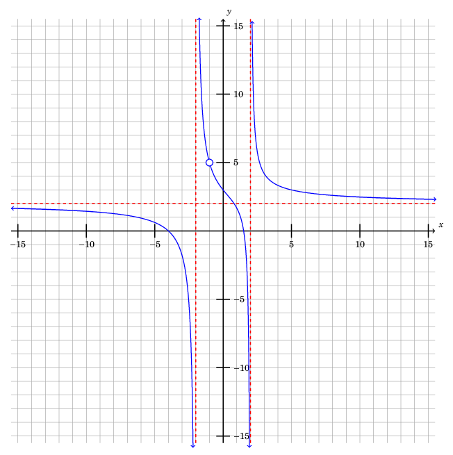
For example, suppose I want to plot $y = r(x)$, where $$r(x) = \frac{6x^3 + 21x^2 - 21x - 36}{3x^3 + 3x^2 - 12x - 12},$$ with $-15.5 \leq x \leq 15.5$. Let’s additionally suppose I want to only see $y$-values with $-15.5 \leq y \leq 15.5$. (In other words, the “viewing rectangle” will be $[-15.5, 15.5] \times [-15.5, 15.5]$.)

Factoring the numerator and denominator, we have:

$$r(x) = \frac{6x^3 + 21x^2 - 21x - 36}{3x^3 + 3x^2 - 12x - 12} $$ $$\phantom{r(x)}= \frac{\left(x + 1\right) \left(2 x - 3\right) \left(3 x + 12\right)}{\left(x + 1\right) \left(x + 2\right) \left(3 x - 6\right)}$$ $$\phantom{r(x)}= \frac{\left(2 x - 3\right) \left(3 x + 12\right)}{\left(x + 2\right) \left(3 x - 6\right)}, \; x \not = -1.$$

As you can see, we will have vertical asymptotes at $x = -2$ and $x = 2$, and a hole at $x = -1$. There will also be a horizontal asymptote at $y = 2$.

To handle the asymptotes, we plot the function $$\hat r(x) = \frac{\left(2 x - 3\right) \left(3 x + 12\right)}{\left(x + 2\right) \left(3 x - 6\right)}$$ along three intervals:

$[-15.5, -2)$,
$(-2, 2)$, and
$(2, 15.5]$

(Actually, for each of the above intervals $I$, we plot something approximating $\left\{(x, \hat r(x)): x \in I \text{ and } |\hat r(x)|\leq 16\right\}$.)

Here is the Python script:

 1
 2
 3
 4
 5
 6
 7
 8
 9
10
11
12
13
14
15
16
17
#! /usr/bin/env python3

import numpy as np

r = lambda x: (2*x - 3)*(3*x + 12)/((x + 2)*(3*x - 6))

xvals = [
        np.arange(-15.5, -2, 0.01),
        np.arange(-2.01, 2, 0.01),
        np.arange(2.01, 15.6, 0.01)
        ]

for idx, interval in enumerate(xvals):
    with open("plot2_{}.table".format(idx), "wt") as outfile:
        for x in interval:
            if abs(r(x)) <= 16:
                outfile.write("{:f} {:f}\n".format(x, r(x)))

Here is the corresponding LaTeX code:

 1
 2
 3
 4
 5
 6
 7
 8
 9
10
11
12
13
14
15
16
17
18
19
20
21
22
23
24
25
26
27
28
29
30
31
32
33
34
35
36
37
38
39
40
41
42
43
44
45
46
\documentclass[border=0.25cm]{standalone}

\usepackage{tikz}
\usepackage{fouriernc}

\begin{document}

  \begin{tikzpicture}[scale=0.5] % Scale keeps the graphic small

    \draw[gray] (-15.5, -15.5) grid (15.5, 15.5);

    % x-axis
    \draw[thick, black, ->] (-15.5, 0) -- (15.5, 0)
      node[anchor=south west] {$x$};

    % x-axis tick marks
    \foreach \x in {-15, -10, -5, 5, 10, 15}
      \draw[thick] (\x, 0.5) -- (\x, -0.5)
        node[anchor=north] {\(\x\)};

    % y-axis
    \draw[thick, black, ->] (0, -15.5) -- (0, 15.5)
      node[anchor=south west] {$y$};

    % y-axis tick marks
    \foreach \y in {-15, -10, -5, 5, 10, 15}
      \draw[thick] (-0.5, \y) -- (0.5, \y)
        node[anchor=west] {\(\y\)};

    % graph of function
    \draw[thick, blue, <->] plot[smooth] file {plot2_0.table};
    \draw[thick, blue, <->] plot[smooth] file {plot2_1.table};
    \draw[thick, blue, <->] plot[smooth] file {plot2_2.table};

    % hole at (-1, 5)
    \draw[thick, blue, fill=white] (-1, 5) circle (2.5mm);

    % vertical asymptotes
    \draw[thick, dashed, red] (-2, -15.5) -- (-2, 15.5);
    \draw[thick, dashed, red] (2, -15.5) -- (2, 15.5);

    % horizontal asymptote
    \draw[thick, dashed, red] (-15.5, 2) -- (15.5, 2);

  \end{tikzpicture}
\end{document}

And here is the result:

Plotting functions that go through certain points: two ways

Suppose I want to plot a function that go through certain points, say:

$(-4, 2)$,
$(-1, 6)$,
$(2, 3)$, and
$(4, 5)$.

I want the function to be differentiable.

Method one: Bézier curves

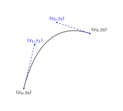
Recall from the last post that a (cubic) Bézier curve is specified by four points:

A start point ($(x_0, y_0)$ in the diagram below)
Two control points ($(x_1, y_1)$ and $(x_2, y_2)$ in the diagram below)
An end point ($(x_3, y_3)$ in the diagram below)

The syntax is: \draw ($x_0, y_0$) .. controls ($x_1, y_1$) and ($x_2, y_2$) .. ($x_3, y_3$);

Now, we can combine multiple Bézier curves into a single \draw. For example, \draw ($x_0, y_0$) .. controls ($x_1, y_1$) and ($x_2, y_2$) .. ($x_3, y_3$) .. controls ($x_4, y_4$) and ($x_5, y_5$) .. ($x_6, y_6$); will produce:

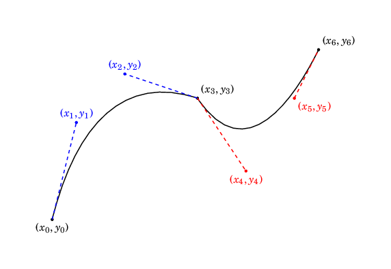
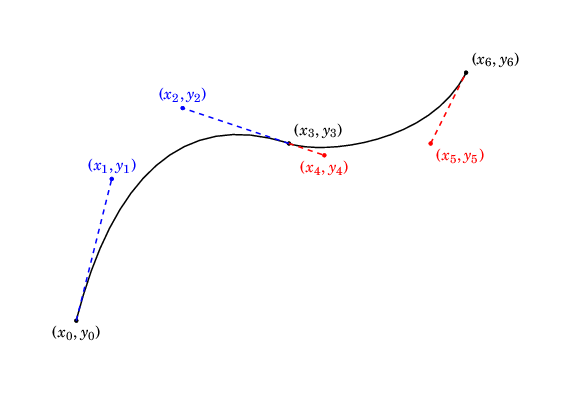
In general, this curve will not necessarily be differentiable. We can get differentiability by ensuring that $(x_2, y_2)$, $(x_3, y_3)$ and $(x_4, y_4)$ are colinear (i.e., the end of the first Bézier curve has the same derivative as the beginning of the second) with $x_2 \not = x_3$:

Keeping these principles in mind, we can plot a function going through the desired points with:

 1
 2
 3
 4
 5
 6
 7
 8
 9
10
11
12
13
14
15
16
17
18
19
20
21
22
23
24
25
26
27
28
29
30
31
32
33
34
35
36
37
38
39
\documentclass[border=0.25cm]{standalone}

\usepackage{tikz}
\usepackage{fouriernc}

\begin{document}

  \begin{tikzpicture}[scale=0.5] % Scale keeps the graphic small

    \draw[gray] (-5.25, 0) grid (5.25, 8.25);

    % x-axis
    \draw[thick, black, ->] (-5.25, 0) -- (5.25, 0)
      node[anchor=south west] {$x$};

    % x-axis tick marks
    \foreach \x in {-5, 5}
      \draw[thick] (\x, 0.25) -- (\x, -0.25)
        node[anchor=north] {\(\x\)};

    % y-axis
    \draw[thick, black, ->] (0, 0) -- (0, 8.25)
      node[anchor=south west] {$y$};

    % y-axis tick marks
    \foreach \y in {4, 8}
      \draw[thick] (-0.25, \y) -- (0.25, \y)
        node[anchor=west] {\(\y\)};

    % graph of function
    \draw[thick, blue, <->] (-5.25, -0.5)
      .. controls (-4, 0) and (-5, 0) .. (-4, 2)
      .. controls (-3.5, 3) and (-3, 6) .. (-1, 6)
      .. controls (1, 6) and (1.75, 4) .. (2, 3)
      .. controls (2.25, 2) and (3, 2) .. (4, 5)
      .. controls (4.5, 6.5) and (4.5, 7) .. (5.25, 8);

  \end{tikzpicture}
\end{document}

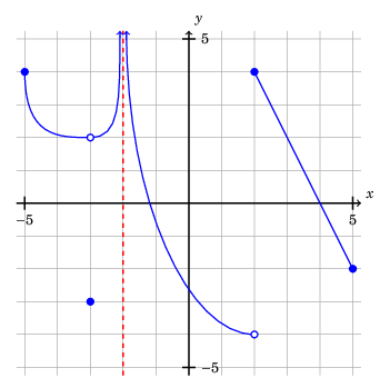
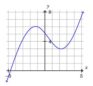
Here is the output:

Method two: Polynomial interpolation

SciPy’s interpolation functionality can find a smooth function that passes through an arbitrary list of points. Here is an example of a Python script to produce such a function and create a table in the necessary format:

 1
 2
 3
 4
 5
 6
 7
 8
 9
10
11
12
13
14
15
16
17
18
19
20
21
22
23
#! /usr/bin/env python3

import numpy as np
import scipy.interpolate

coords = [(-10, 8), (-4, 2), (-1, 6), (2, 3), (4, 5), (10, 1)]
# Since our goal is to plot from x = -5.25 to x = 5.25,
# we need to specify some points beyond that interval on both sides.

xcoords, ycoords = zip(*coords)
# This produces a seperate list of x-coordinates and y-coordinates

f = scipy.interpolate.interp1d(xcoords, ycoords, kind="cubic")

xvals = np.arange(-5.25, 5.25, 0.01)
yvals = f(xvals)

outcoords = zip(xvals, yvals)
# This produces a list of coordinate pairs

with open("plot3.table", "wt") as outfile:
    for pair in outcoords:
        outfile.write("{:f} {:f}\n".format(pair[0], pair[1]))

Note that if we had set coords = [(-4, 2), (-1, 6), (2, 3), (4, 5)], then the resulting function would not have had a defined value outside of the interval $[-4, 4]$.

To plot, we use the following tikzpicture:

 1
 2
 3
 4
 5
 6
 7
 8
 9
10
11
12
13
14
15
16
17
18
19
20
21
22
23
24
25
26
27
28
29
30
31
32
33
34
\documentclass[border=0.25cm]{standalone}

\usepackage{tikz}
\usepackage{fouriernc}

\begin{document}

  \begin{tikzpicture}[scale=0.5] % Scale keeps the graphic small

    \draw[gray] (-5.25, 0) grid (5.25, 8.25);

    % x-axis
    \draw[thick, black, ->] (-5.25, 0) -- (5.25, 0)
      node[anchor=south west] {$x$};

    % x-axis tick marks
    \foreach \x in {-5, 5}
      \draw[thick] (\x, 0.25) -- (\x, -0.25)
        node[anchor=north] {\(\x\)};

    % y-axis
    \draw[thick, black, ->] (0, 0) -- (0, 8.25)
      node[anchor=south west] {$y$};

    % y-axis tick marks
    \foreach \y in {4, 8}
      \draw[thick] (-0.25, \y) -- (0.25, \y)
        node[anchor=west] {\(\y\)};

    % graph of function
    \draw[thick, blue, <->] plot[smooth] file {plot3.table};

  \end{tikzpicture}
\end{document}

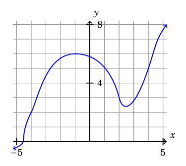
Here is the result:

As we have seen, creating plots with TikZ allows you a deep amount of control over the final result, and can be especially powerful when combined with a programming language such as Python.