Plots from the lecture on the logistic equation

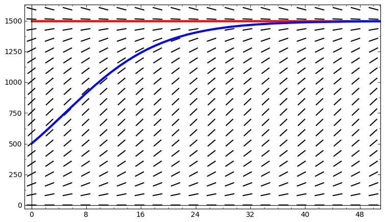
The differential equation \(\frac{dy}{dt} = 0.2y\left(1 - \frac{y}{100}\right)\)

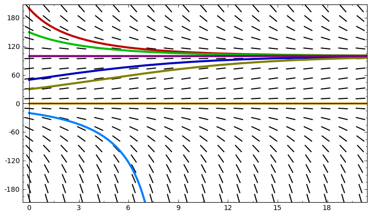
Above is a slope field for the logistic differential equation \[\frac{dy}{dt} = 0.2y\left(1 - \frac{y}{100}\right),\] as well as plots of several different solutions. Note that equillibrium solutions at $y= 100$ and $y = 0$. As you can see, if $y(0) > 0$, we have \[\lim_{t \rightarrow \infty} y(t) = 100.\] On the other hand, if $y(0) < 0$, then there is some value $t_b > 0$ for which \[\lim_{t \rightarrow t_b^-} y(t) = -\infty.\]

Fish example

Above is the a slope field for the logistic differential equation \[\frac{dy}{dt} = 0.14163 y \left(1 - \frac{y}{1500} \right),\] along with a plot (blue curve) for the particular solution \[y(t) = \frac{1500}{1 + 2 e^{-0.14163 t}}.\] As you can see, the fish population begins at $y(0) = 500$ and increases toward the carrying capacity 1,500.