Plots from the lecture on first-order linear differential equations

Tank example

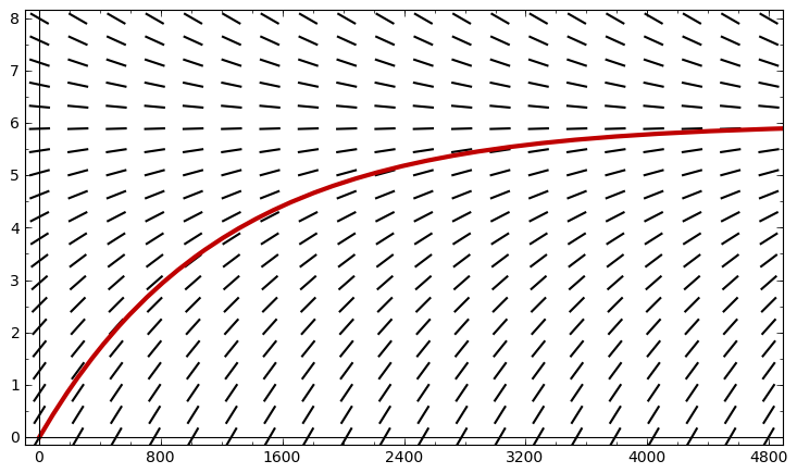
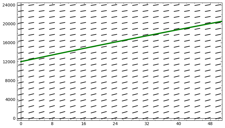
The mass (in grams) of the salt in the tank $y(t)$ the differential equation \[\frac{dy}{dt} = 240 - \frac{y}{200 + t},\; t \geq 0,\] and the initial condition $y(0) = 12000$. The solution to this differential equation satisfying the initial condition is \[y(t) = 120(t + 200) - \frac{2400000}{t + 200}, \; t \geq 0.\] Here, we see a slope field for the differential equation, along with our particular solution:

The concentration of salt is $c(t) = y(t)/(2t + 400)$. Here is a plot of $c(t)$:

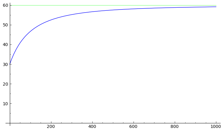
As you can see, $\lim_{t \rightarrow \infty} c(t) = 60$. This makes sense, because the incoming mixture has a concentration of 60 g/L, and in the long run, most of the water will have come from the incoming mixture.

Polluted pond example

The concentration (in g/m³) of toxin in the pond $c(t)$ satisfies the differential equation \[\frac{dc}{dt} = \frac{1}{200} - \frac{c}{1200}, \; t \geq 0,\] and the initial condition $c(0) = 0$. The solution to this differential equation satisfying the intitial condition is \[c(t) = 6 - 6 e^{-t/1200}.\] Here is a slope field for the differential equation, along with our particular solution:

As you can see, $\lim_{t \rightarrow \infty} c(t) = 6$. Again, this makes sense, because the incoming water has a toxin concentration of 6 g/m³, and in the long run, most of the water in the pond will have come from the polluted stream.