Forced vibrations

This example illustrates the relationship between the solution
 of a differential equation modeling forced vibration and the forcing function. Here we consider the
 initial value problem y′′+0.125y′+y= 3cos(ωt),y(0)=0,y′(0)=2.
 In blue is the solution to the IVP, while in red is the forcing function F(t)=3cos(ωt).
 Here you can see how
 different values of ω affect the amplitude of the solution.
Here are plots for various values of ω: 

ω=0.3

ω=1

ω=3

Here is an animation showing the solution for many values of ω:

This example illustrates periodic variation of amplitude which occurs when you have a forced, 
 undamped vibration. Suppose a vibration is modelled by y′′+y′=cos(ωt),y(0)=0,y′(0)=0.
 Then the solution will be y=(21−ω2sin(2(1−ω)t))sin(2(1+ω)t). 
 If ω is close to 1, then 1−ω  is small, and hence the factor sin(2(1+ω)t) 
 is oscillating much faster than 21−ω2sin(2(1−ω)t). 
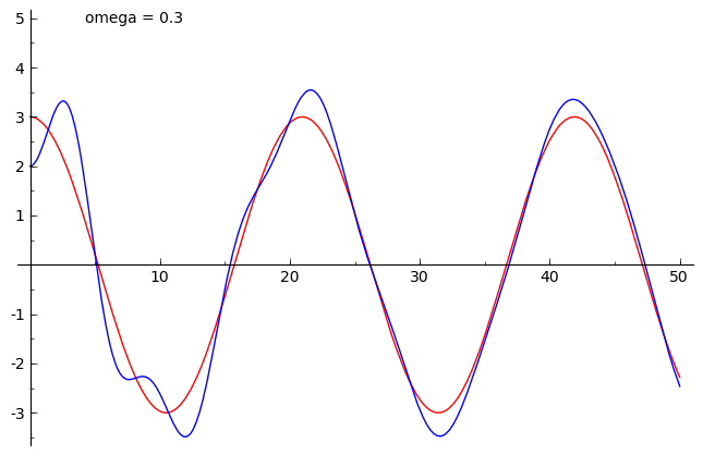
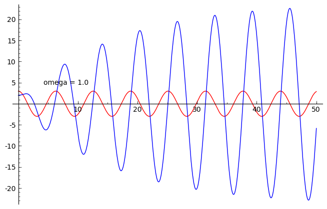
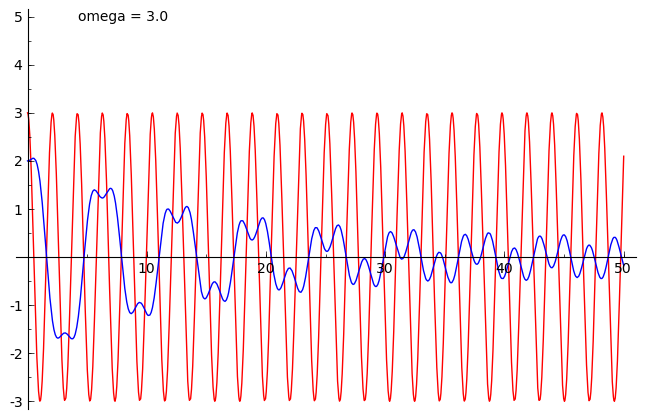
 So, we think of | |  21−ω2sin(2(1−ω)t)| |    (shown in red) as periodically varying the amplitude of the sine curve.
Here are plots for various values of ω:

ω=0.7

ω=0.9

ω=0.95

Here's an animation showing the solution for many values of ω: